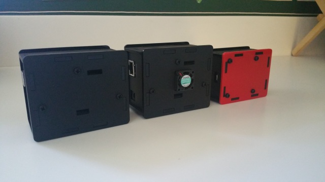
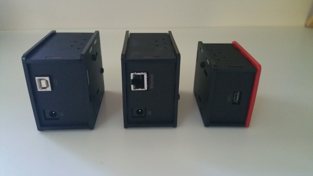
In the previous post I talked about how I built Pickle Jr – which is my name for the networked air pollution monitor that comprises the Shinyei PPD42 with a small Sunon fan fused to the 42. I first built the Pickle described earlier which was the networked air pollution monitor that comprised the PPD60PV-T2 (aka T2) with a small fan fused to it and an Arduino Ethernet.
I decided to do make the Pickle Jr. hoping that the same improvement in noise and sensitivity I got with the Pickle (T2) would also apply to the 42.
For those who have worked with the 42 or one of its cousins (the DSM501 and the Sharp GP2Y thingy) know that the data gives many many zeros. As in this blog post from Darrell Tan in Singapore. http://irq5.io/2013/07/24/testing-the-shinyei-ppd42ns/, and in this blog from David Holstius http://www.davidholstius.com.
That is even when there is known air pollution, the sensor reads zero. If you wait long enough or average over a long time then there is some data. But waiting for an hour, or in some cases the entire day is not that great so I wanted to see results with a minute or so. So I added the fan to the 42 and measured it against the 42 without the fan, and the T2 and the AES-1, the zeros improved, but unfortunately I still got many of them (this is with PM2.5 less than approx 25 ug/m3.). The issue with the zeros is that the data cannot be scaled because a zero is a zero 🙂 So I have seen other folks use a previous non-zero value to guess what that zero should have been. But what if you could reduce the number of zeros significantly in the first place ?
So how do I reduce the number of zeros ?? The 42 has two controls on the board that are set at the Shinyei factory for calibration. I did not want to mess with those if I could help it because it would be impossible to know precisely what I had set them to in case I (or others) wanted to do the same thing. Then I found this brilliant note by Tracy Allen and he has figured out how the 42 works!
http://takingspace.org/wp-content/uploads/ShinyeiPPD42NS_Deconstruction_TracyAllen.pdf
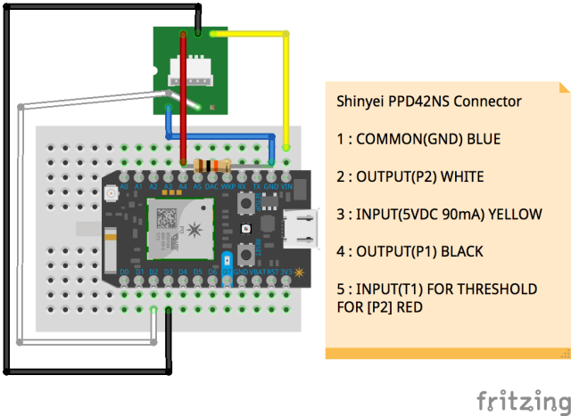
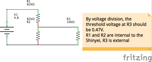
After reading and re-reading the note (with help from others), I understood that P1 is what most of us measure and that P2 is less sensitive. But, we can make P2 more sensitive by decreasing the threshold voltage at Pin5. I did not know quite how to do that right away but after some trial and error, I attached a 10 KΩ resistor between Pin5 and Ground and then measured the voltage at that Pin. Why 10 KΩ ? Because I wanted to reduce the threshold to half from what it was for the P1. I measured 1.35V as the threshold for P1 and with the 10 KΩ resistor I measured 0.491V at Pin5. Without the resistor I measured 2.48V at Pin5.
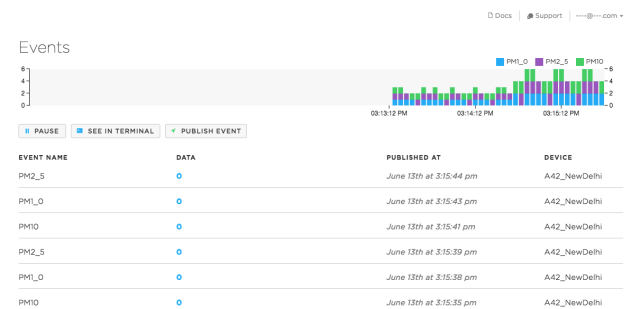
So now with the fan and with the resistor I measured both P1 and P2.
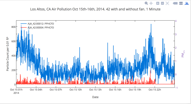
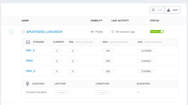
The sensor 42:00012 is the 42 with Fan and resistor and 42:00004 is the vanilla 42. As before I store all the data in tempoiq and make all the plots with plotly. I have written the code to store and extract info from tempoiq and then post process in plotly. The y-axis is just the P1 and P2 voltages scaled by a straight line curve from the Shinyei data sheet measured every minute. The x-axis is the date. So now the number of zeros has gone down dramatically! But obviously the calibration would be quite off. However, since I did not muck around with the two controls, if all of us used the same resistor value then we could come up with a *new* calibration curve (more on this later).
Now how good is this 42 with fan and resistor, let me call this 42FR compared to the T2 with fan or the Dylos ? I wanted to do this with the AES-1 as well, but the windows computer it is connected to has some issues. So here is the 42FR, 42 and Dylos with measurements every minute:
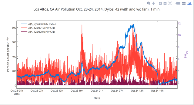
The 42FR is still quite noisy but has a response that generally traces the Dylos over this per minute interval. Changing the interval to 10 minutes results in
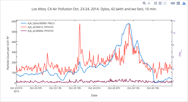
Now the respond of the 42FR vs the 42 is much clearer wrt the Dylos. Adding the T2 with fan to the mix for 1 minute intervals gives:
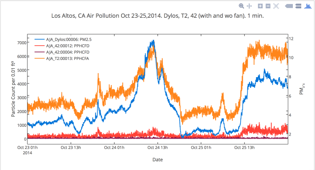
Since I used the left y-axis for both the T2 and 42’s, the latter look “compressed” and, of course, the T2 with fan tracks quite closely to the Dylos. BTW, this is not the calibrated particle counts, I have not done that yet as I said before. Here is the same data over 10 minute intervals
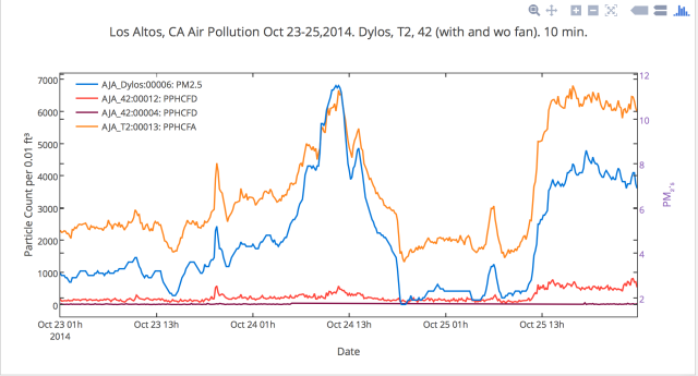
Interestingly the vanilla 42 can barely be seen wrt the 42FR. And now the proof of the pudding, that is how is the regression of the 42FR and the vanilla 42 vs the T2 with fan and the Dylos. First the comparisons with the T2
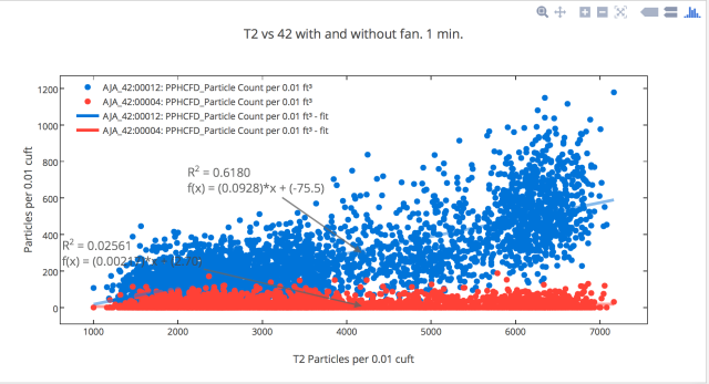
That is a pretty decent R2 of 0.62 for the 42FR compared to an R2 of 0.02 for the vanilla 42! Across 10 minutes it becomes better
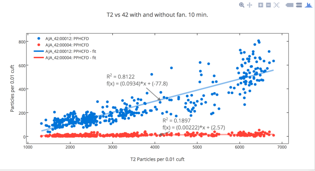
R2 of 0.81 for the 42Fr compared to an R2 of 0.19 for the vanilla 42. But the number of points are not enough, I need to continue this for a longer period. Next is the comparisons to the Dylos, first the per minute

A lower R2 than for the T2 but still oodles better than the vanilla 42. And finally the same over 10 minute intervals
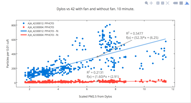
A decent R2 of 0.55 for the 42FR vs 0.21 for the vanilla 42.
I absolutely love tempoiq and plotly. I am so thankful to the tempoiq guys who have just rocked for this project! And the plotly tool is the greatest too.
Work still to be done (likely in the holiday break): compare with much higher PM2.5 concentrations, and then produce a calibration curve of the 42FR vs Dylos and T2 that anyone can use if they want to modify their 42’s. As a summary, the mods are to add a fan to the plastic housing and the resistor to the threshold pin Pin5.